The Paradox of Enrichment: The Theory

WARNING: This post contains calculus, phase planes, time series and other mathematical concepts that may be horrifically boring to the non-mathematically inclined. Reader discretion is advised.

A Short Aside: Exponential and Logistic Growth

Before I get into the hot and heavy mathematics and theory behind the paradox of enrichment, I thought it would be a good idea to introduce two fundamental equations of ecology: the exponential and logistic growth curves. While many people have heard of exponential growth as it is used in many fields, logistic growth is usually restricted to ecology.

Exponential growth is normally formulated and derived in the following way:
the rate of growth of a population N, dN/dt, is proportional to that population. In order to make proportionality explicit, we introduce a proportionality constant, r. Therefore, we have the following equation:

dN/dt= rN

While this is all nice and dandy, what us crazy ecologists normally want to know is what will the population size be at any instant of time, if we know the starting population size and the rate of growth. To do that, we are going to have to do some intergration (yay, calculus). First, let us rearrange the equation:

dN/N = rdt, then lets do the intergration and the algebra:


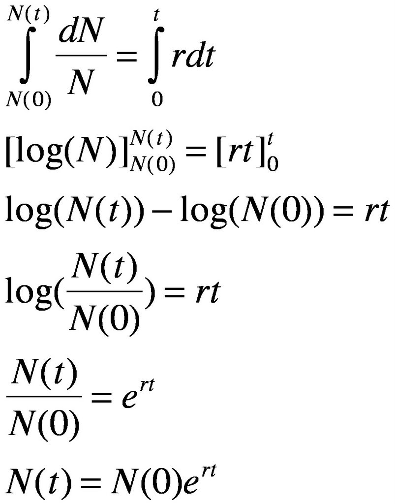
And now we have a general equation for exponential growth. However, if things in nature grew exponentially, then the world would be covered in an immense blob of bacteria. Therefore, there must be some sort of regulation or limitation (important distinction here, regulation means density-dependent effects, such as predation, disease, food, while limitation means density-independent factors, such as temperature, water salinity and other such factors) acting on the population. Let us assume that density-dependent factors are regulating population size. Therefore, in a certain environment, our organism of interest has a limit to its maximum sustainable population size. We shall call this population size the carrying capacity of the environment for the organism of interest. We shall symbolize the carrying capacity by the parameter K in our model. Therefore, adding K into our previous equation for exponential growth, we obtain the following:

dN/dt = rN (1- N/K)


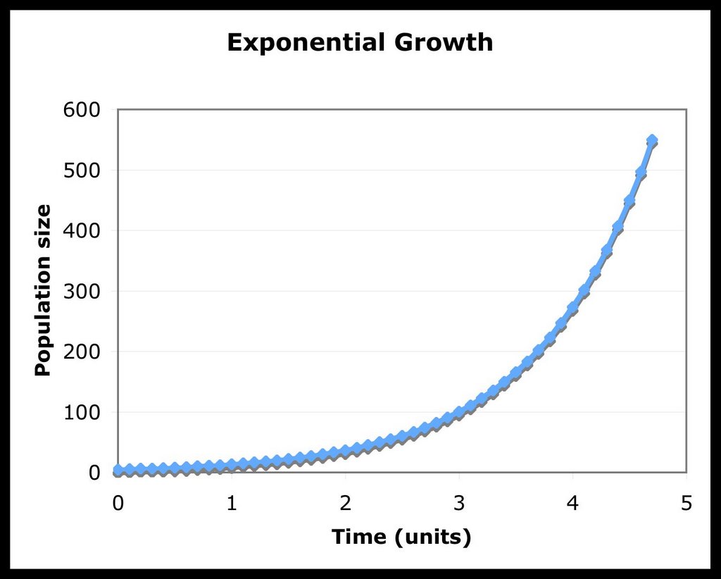
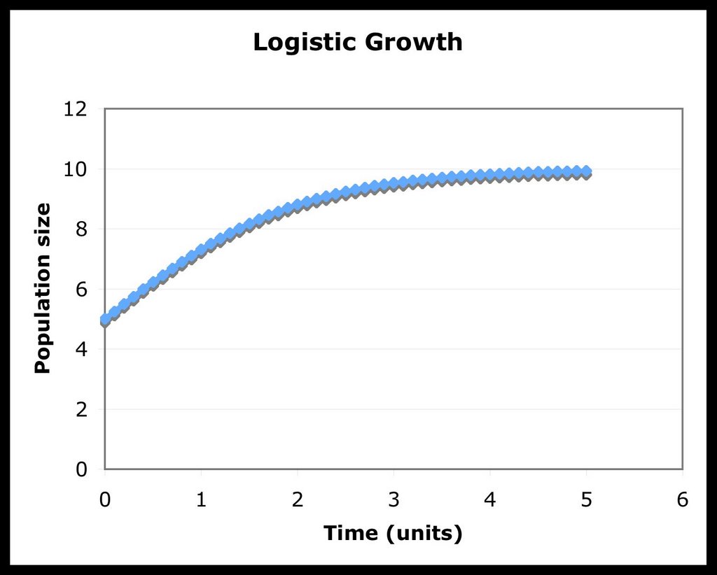
As we can see, when the population reaches the size of K (when N=K), the rate of growth is 0. Also, if the population started at a size greater than K (No > K), there would be a negative growth rate till the population reached the carrying capacity. Here are two graphical examples, showing the differences between exponential and logistic growth when the initial value of N is 5, r is 1 and K is 10:


Now, let us derive a general solution for this differential equation. It is a bit more tricky than the solution for exponential growth, so try to follow along:








(Note: At one point, I used partial fraction in order to simplify the integral. Solving partial fractions are relatively easy. In the above example, we had 1= A(1-x) + Bx after we multiplied both sides by x(1-x). We then look at the case when x=0, so
1=A(1-0) + B*0 -> 1=A. Next, we look at the situation where x is not equal to zero, so 1= A - Ax + Bx. Since we know that A=1, then 0= Bx - Ax -> B=A=1.)

And now we have a solution for logistic growth. Wasn't that fun? Wow, my short asides are gigantic... I guess I'll never get published in Nature with such a verbose writing style, but that's their lost. Anyways, back to the topic at hand.

Lokta-Volterra Equations for Predator-Prey Dynamics

In the aside, we discussed the case of the population dynamics of a single species. What would happen if we had two species interacting, say a prey and a predator species? The simplest way of formulation such a situation mathematically is the Lokta-Volterra Equations:



Where N is the prey population, P is the predator population, r is the prey's growth rate, a represents the uptake of the predator of the prey, e is the efficiency of the predator in turning prey biomass into predator biomass and m represents the mortality rate of the predator.

The two main assumptions of these equations is that the prey population would grow exponentially if the predator was absent and that the predator consumes the prey with a linear functional response, i.e. the more prey around, the more prey are consumed by the predators.

So what do we want to know about our predator-prey model we just formulated? A good way to start is to see when our populations of predators and of prey are stable, i.e. when dN/dt and dP/dt are equal to zero at the same time, as these are coupled ordinary differential equations.







































Alright, first off, we solve the equations, just like we did for exponential and logistic growth. Note that my formula and the formula used in the graphic are functionally equivalent. The only difference is that we used different letters for the constants.

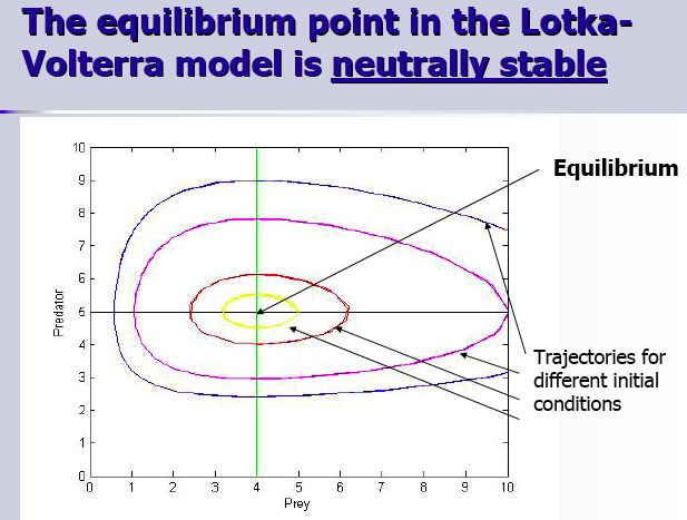
Next, we plot the solutions of these equations on a phase plane. A phase plane helps one visualize where the rates are equal to zero as well as determining the flow (the growth and number) of the differential equations (populations). When making a phase plane in two dimensions, one normally plots the equilibrium solutions of the differential equations one at a time, then one see on which part of the phase plane would dH/dt (the prey) be bigger or smaller than zero. When dH/dt is greater than zero in a certain region of the phase plane, the flow will be in the positive direction of H (goes to the right). If dH/dt is less than 0 in a certain region of the phase plane, then the flow will go towards negative values of H (goes to the left). On the above diagrams, dH/dt=0 is the horizontal line and dH/dt>0 is below it and dH/dt<0 is above it. For dP/dt (the predator), it is the same principle. On the diagrams, dP/dt=0 is the vertical line, with dP/dt<0 to the left of the isocline and dP/dt>0 to the right of the isocline.

Our stability analysis using isoclines has shown that the predator and prey isoclines are both straight lines and where they will intersect will be the fixed point (a fixed point is a point where the predator and the prey populations do not change over time, i.e. the populations are in stable equilibrium). If one starts with either population away from their fixed point value, then the populations will oscillate around the fixed point forever (this can be seen from the fact that the the trajectories of the flow are closed loops). Therefore, the fixed point is neutrally stable, as the fixed point neither attracts nor repulses the the flow. This also means that the initial conditions of the system determine the length and amplitude of the cycles for an eternity, unless it gets perturbed. If perturbed, it will then go to another neutrally stable cycle. However, in nature, there seems to be populations that show more stable equilibrium dynamics as well as fairly stable cycles that return to those states when perturbed. Therefore, the Lotka-Volterra model of predator-prey dynamics are grossly irrealistic. So how can one improve on the system?

Rosenzweig-MacArthur Model of Predator Prey Dynamics

Well, one way of doing it would be to incorporate more realistic assumptions in the formulations of the equations. Most likely, there would be some density-dependence on the prey, resulting in logistic growth if the predator was absent. In addition, it would be more realistic if the predator could become satiated with prey (i.e. one predator surrounded by one thousand prey items cannot keep consuming at a linear rate, i.e. if there are two prey around, the predator would eat one, if there are 4 prey around, the predator would eat two... if there are 1000 prey around, the predator would eat 500 seems a bit crazy). Rosenzweig and MacArthur created such a model and analyzed its properties:


































Now you might be wondering what Type II means in the equations. Well, it means that we have changed the Type I (linear) functional response for the Hollings Type II functional response (non-linear, asymptotic). I'll go into greater detail about it at a later date as this post is already gigantic. In any event, all one needs to remember is that these changes have great consequences on the dynamics and the stability of the system. First off, their are multiple kinds of stability: We can have a stable fixed point, a neutrally stable fixed point and a unstable fixed point surrounded by a stable limit cycle. These dynamics are fundamentally different from the Lotka-Volterra system. This is mostly do to the shape of the prey isocline and the location of the predator isocline. If the predator isocline is to the right of the maximum (as in the summit of the inverse parabola) of the prey isocline, then there will be a stable fixed point. If the predator isocline is exactly on the maximum of the prey isocline, one would get a neutrally stable fixed point like the Lotka-Volterra system. If, however, the predator isocline is on the left of the maximum of the prey isocline, then the fixed point will be unstable (i.e. repulsive) while a stable limit cycle (the flow goes towards a closed loop) will form around it. If the predator isocline is very far to the left of the maximum, then large oscillations going towards the limit cycle will occur, leading to population levels near zero, hence extinction.

Nevertheless, one may be wondering after all this time spent on these varioius equations and models, what does all this have to do with the Paradox of Enrichment? Well, the link between the Rosenzweig-MacArthur model and the paradox is based upon the carrying capacity, K. As you already know, K is supposed to represent the amount of nutrients in the system available to the prey to grow. Changing the value of K changes the shape of the prey isocline. In fact, what it does, for the most part, is to move the maximum over to the right. Therefore, if one increases K from 3 to 4, as in the diagram above, one can see that the system goes from stable equilibrium to unstable equilibrium. These unstable equilibriums can be more prone to extinction as they undergo oscillations. Therefore, if one increases K, then one also increases the risk of extinctions, reducing the diversity of the system, even though there are more nutrients, hence more individuals could be potentially supported in the area!

So there you have it. The theory behind the original formulation of the Paradox of Enrichment. Of course, this is an extremely simple model and its dynamics are probably irrealistic as well. Nevertheless, there are many natural phenomena that seem to vindicate its main predictions. That will be the next topic explore in this opening series of articles about this blog's namesake.

Note: All figures and diagrams, except for the plain text equations (made by Equation Marker) and the logistic and exponential curves, were taken from lecture 14 of Biology 308: Ecological Dynamics, taught by Gregor Fussman.